
 Best Platforms
 Live Odds








11 Accuracy Metrics for Senate Forecasts to Evaluate in 2026
Score 2026 senate forecasts with Brier/log loss, RPS, CRPS, interval/coverage checks, plus a snapshot protocol and calibration diagnostics.
You’re trying to figure out which Senate forecast to trust before you act on it. The obvious approach—“who’s ahead” or “who called more races”—breaks down fast when some sources publish probabilities, others publish rating buckets, and others publish seat distributions that don’t resolve to the same thing.
This case study gives you a clean way to score them anyway: define what counts as the forecast and what counts as the truth, take consistent snapshots into an archive, map each forecast format to the metrics that actually apply, then use a short diagnostic checklist to decide what to follow, what to fade, and what to treat as signal—not probability.
Forecasts vs truth
Accuracy work starts before you compute a single metric. You need a clean set of forecast–outcome pairs, and that means being explicit about (1) what your “Senate forecast” object is and (2) what counts as the “truth” it resolves to.
For 2026, you’re ultimately anchoring everything to realized election outcomes from a cycle with 35 Senate seats up (33 regular elections plus 2 specials in Ohio and Florida) on November 3, 2026. But different products slice that reality into different “questions,” and you can’t score them as if they were the same question.
Forecast objects
- Race win probability (one seat): A number like “Dem wins Ohio: 0.62.” Your truth is a single 0/1 outcome for that race (who won that seat).
- Chamber-control binary (one contract): A yes/no proposition like “Party X controls the Senate.” Your truth is whatever the market/contract says “control” means at settlement—not your preferred political definition.
- Rating bucket (ordered categories): Labels like Safe/Likely/Lean are categorical forecasts. For example, one widely used map defines Lean as 60%+, Likely as 75%+, and Safe as 95%+, and it refreshes on a daily 6:00 PM Eastern schedule. Your truth is still the race winner, but your dataset must preserve the bucket (not pretend it was a probability).
- Seat-count distribution (whole chamber): Simulation-driven outputs (e.g., 50,000 daily simulations) produce a distribution over seat counts. Your truth is the realized seat count after the election is decided for the seats being modeled.
Resolution semantics
A resolution rule is the contract/product’s definition of what event occurred, and it decides what you’re allowed to treat as ground truth.
That difference is not theoretical. Kalshi’s Congressional Control Contracts are cash-settled binaries whose settlement is determined by the party affiliation of the chamber leader on the expiration date; for the Senate, that leader is the President Pro Tempore. On the “Which party will win the U.S. Senate?” market page, the contract can open Nov 3 (8:00am EST) yet reference a later date (e.g., Feb 1, 2027) for settlement context.
If you score “control” using election-night seat majority while the contract settles on leadership at expiration, you’re not measuring forecast accuracy—you’re measuring how often you overrode the rules. Decide your resolution semantics first, then every forecast snapshot can be paired to a single, unambiguous truth value.
Snapshot and archive (2026 protocol)
A “snapshot” is one frozen copy of a forecast as it existed at one timestamp. If you can’t reproduce snapshots, you can’t build clean forecast–outcome pairs without cherry-picking.
Treat each snapshot as an auditable record with (a) an unambiguous time, (b) an unambiguous forecast object, and © an unambiguous resolution target. The goal is that someone else can rerun your collection rules and get the same set of rows—then your accuracy metrics are just arithmetic.
- Define the snapshot clock before you look at any numbers. Write down one rule for when a snapshot is taken and stick to it for the entire cycle.
- Use a single time standard: store times in UTC.
- Use one trigger: either a fixed schedule (e.g., “daily at 00:00 UTC”) or the publisher’s displayed update moment. Don’t mix them.
- Record two timestamps every time:
observed_at_utc: when your collector fetched the page/API.as_of_utc: the forecast’s own “Last updated” timestamp when it’s visible on the page (MarketsPrediction displays “Live Data” with a visible “Last updated” time).- If the page doesn’t expose an “as of” time: keep
as_of_utcblank and rely onobserved_at_utc—but don’t backfill or infer it later.
- Freeze the forecast object exactly as displayed. Save enough that a third party can verify what you saw without trusting your parsing.
- Raw capture: store the exact payload you ingested (HTML and/or JSON), plus request URL and query parameters.
- Rendered capture: store a screenshot or print-to-PDF of the rendered view that shows the numbers you extracted.
- Parsing trace: store the selectors/JSON paths (or equivalent) you used to extract the probability/bucket/distribution so a reviewer can reproduce your extraction from the raw payload.
- Store market/contract metadata alongside the odds. Odds aren’t interpretable without the instrument definition that constrains them.
- For Kalshi Congressional Control Contracts, archive the contract mechanics (e.g., the $0.01 tick size, the $0.01–$0.99 listing band, and the $1 notional) because these define what “the price” can be and how rounding should be handled in your dataset. (See Kalshi’s CONTROL product certification: https://kalshi-public-docs.s3.amazonaws.com/regulatory/product-certifications/CONTROL.pdf.)
- Persist the market identifier and the exact contract/outcome label text as displayed, not just a human nickname you make up later.
- Capture context fields that drift. Archive any on-page fields that can change over time or disappear later, so you can audit what information was available at the moment of the snapshot.
- Examples: displayed volume, liquidity/open interest fields, end date/expiration, and any visible “rules” or settlement snippets on the page.
- Store these as separate columns (don’t bury them only in screenshots) so you can filter/QA later (e.g., detect venue changes, contract relistings, or rule-text edits).
- Log the resolution pointer you intend to score against. A forecast is only scoreable relative to a precisely identified “truth.” Store that truth target up front and link it to every snapshot.
- Resolution ID: create a stable identifier like
venue:event_slug:contract_id:resolution_version. - Resolution source: store the exact resolution rule text you are using (copy/paste it into your archive) and the URL it came from.
- Resolution date reference: store the specific expiration/settlement date reference used by the contract. For example, Kalshi’s Congressional Control Contracts settle based on the party affiliation of the chamber leader on the expiration date; for the Senate this leader is the President Pro Tempore (https://www.cftc.gov/sites/default/files/filings/documents/2023/orgkexkalshiordersig230922.pdf).
Once this is in place, scoring becomes a bookkeeping exercise, not an argument about timing.
Formats-to-metrics map
Pick metrics that match the output type of the senate forecasts you’re scoring. Otherwise you’ll reward (or punish) a forecaster for something they never claimed to predict.
| Forecast format | What the forecast outputs | Smallest valid metric set | Don’t score it with |
|---|---|---|---|
| Binary win odds | Single probability p(Yes) | Brier or log loss (binary proper score) + calibration check | % correct only |
| Ordered rating buckets | Ordered labels (e.g., Safe→Toss-up) | RPS (ordered-category proper score) | Treating buckets as p |
| Simulated seat distribution | Full distribution over seat counts | CRPS (distribution proper score) | Single-point error |
| Seat interval / range | Central interval (l,u), e.g., “+2–4 seats” | Interval score + interval coverage | CRPS (no distribution) |
| Binary odds (rank-only use) | Same as win odds, but you only care about ordering | ROC/AUC (discrimination only) | Using AUC as “accuracy” |
Log loss is unbounded: if a forecaster ever publishes p=0 for an outcome that happens, the score becomes infinitely bad, so you need to audit for literal zeros before you compute it.
The 11 metrics
Most evaluation should start with a strictly proper scoring rule—a scoring rule where a forecaster maximizes expected score only by reporting their true probability distribution—because it rewards honest probabilities, not just confident ones.
For binary race or chamber-control odds, the workhorses are the Brier score (mean squared error between predicted probability and the 0/1 outcome) and log loss (based on log(p) assigned to what happens; it punishes near‑zero probabilities on realized outcomes very heavily). Log loss is also unbounded (it becomes infinitely bad at p=0), which is why some evaluators prefer the bounded, more interpretable Brier score even if it’s less brutal on extreme misses.
For distributions and buckets, use CRPS (a proper score for full predictive distributions/CDFs), interval score (rewards narrow prediction intervals but penalizes outcomes outside), and RPS (compares cumulative probabilities across ordered categories).
| Metric | What to measure | How to interpret the score (diagnosis) | Valid for which Senate forecast formats |
|---|---|---|---|
| Brier score | Mean (p−y)² over races | Lower better; punishes overconfidence symmetrically | Binary win odds; chamber-control binary |
| Log loss (logarithmic score) | Mean −log(p(realized)) | Lower better; brutal on “near-zero but happened” | Binary win odds; chamber-control binary |
| CRPS | CRPS(F,x) for seat-count CDF F | Lower better; distribution accuracy across all thresholds | Seat-count distribution (simulations/CDF) |
| Interval score (Winkler family) | (u−l)+outside-penalties at α | Lower better; narrow wins, misses hurt a lot | Seat interval / range forecasts |
| Ranked probability score (RPS) | Cum-prob squared gaps vs observed bucket | Lower better; 0 is perfect | Ordered rating buckets; ordered bins |
| Quantile score (pinball loss) | Loss for stated p-quantile of seats | Lower better; under/over misses penalized asymmetrically | Seat quantiles (median, P10/P90, etc.) |
| Prediction interval coverage | Share x ∈ [l,u] at nominal 1−α | Too low: overconfident; too high: too cautious/wide | Seat intervals; any interval forecast |
| ROC/AUC | AUC from ROC curve across thresholds | Higher better (0.5 no skill, 1 perfect); ranking only | Binary odds when you only care about ordering |
| % correct (winner-pick hit rate) | Share of races where p>0.5 side wins | Can be dominated by favorites and hide miscalibration | Binary odds; buckets (after thresholding) |
| Mean absolute error (MAE) | Mean abs(p−y) over races | Lower better; less punishing of extreme misses than Brier | Binary win odds; chamber-control binary |
| Skill score vs baseline | Relative improvement vs baseline score | Not strictly proper even when built from a proper score; use as secondary normalization | Any forecast where base score is defined |
Diagnostics that matter
Proper scores will rank your senate forecasts, but they won’t always tell you why—and with a single Senate cycle you’re working with a small set of resolved events, so a clean-looking ranking can be fragile.
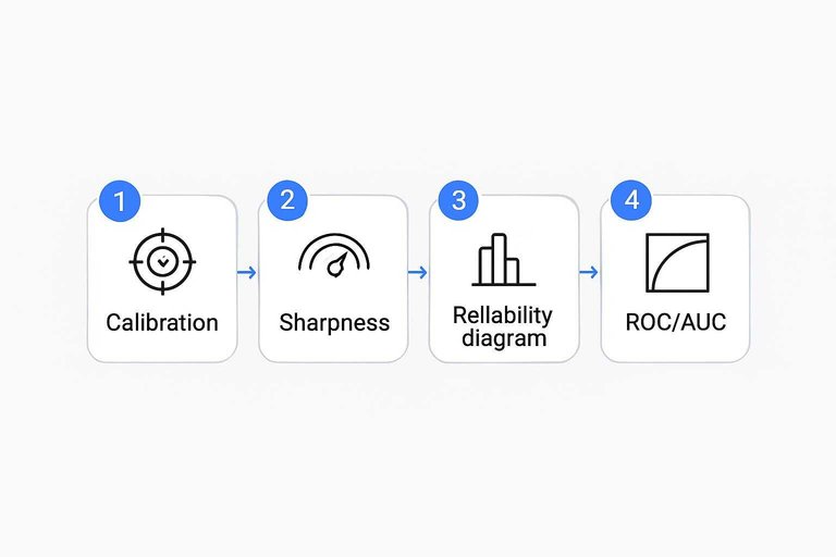
Start by separating calibration—whether events you assign probability p happen about p fraction of the time, over many forecasts—from sharpness, which is how concentrated (confident) your predictive distributions are even before you check if they’re right. In the probabilistic forecasting framework of Gneiting & Raftery, the goal is blunt: maximize sharpness subject to calibration.
To see calibration failures, use a reliability diagram (a binned plot that compares predicted confidence to empirical accuracy). It bins predictions by stated probability, then compares each bin’s average confidence to what actually happened; perfectly calibrated forecasts sit on the identity line. If you need a single summary number, Expected Calibration Error (ECE)—a weighted average of bin-by-bin accuracy–confidence gaps—compresses the diagram into one scalar:
ECE = Σm (|Bm|/n)·|acc(Bm) − conf(Bm)|.
Then sanity-check discrimination separately. ROC/AUC is built from a ROC curve that plots hit rate against false alarm rate across probability thresholds; the AUC summary score runs from 0.5 (no skill) to 1 (perfect). It can look strong while staying almost silent about whether your 0.70s behave like 70%, which is how a forecaster can rank outcomes well while still being miscalibrated.
When metrics disagree, treat that as signal: you’re looking at ranking skill, probability quality, and confidence tightness pulling in different directions.
Make the call
-
Pick one “decision metric” per forecast object. Use a strictly proper score (Brier/log loss for binary odds; RPS for rating buckets; CRPS for seat distributions; interval score for ranges) and rank sources within the same object type.
-
Gate the ranking with calibration, not vibes. Treat calibration (consistency between forecasts and outcomes) as a pass/fail check, and treat sharpness (how concentrated the forecasts are) as a preference only after calibration clears. (That’s the separation Gneiting & Raftery emphasize.)
-
Classify each source into one of three actions.
- Follow: top-ranked proper score and calibration looks clean.
- Fade: good-looking headline rank, but repeated overconfidence signals (e.g., reliability curve off the identity line).
- Signal, not probability: strong discrimination but weak calibration—e.g., good AUC (ranking) even though the probabilities aren’t trustworthy; AUC runs from 0.5 (no skill) to 1 (perfect) and doesn’t “fix” biased probabilities.
-
Publish a minimal performance row you can rerun weekly. Use one row per (source × object):
Source | Object | Primary score | Calibration check | Sharpness/coverage | AUC (if used) | Notes (resolution rule, snapshot clock) -
Lock the rule, then just re-score. If your decision flips often, you’re seeing small-sample fragility—not a stable edge.
Score forecasts the way they resolve
If you want a Senate forecast you can actually trust (or trade against), stop treating every source as if it answered the same question. Lock the resolution semantics and a non-negotiable snapshot clock, then grade each forecast object with the strictly proper score it earns (Brier/log loss for binaries, RPS for buckets, CRPS for seat distributions, interval score for ranges). Use calibration as the gate—reliability diagram/ECE first, sharpness only after—and let discrimination (AUC) tell you “signal” without pretending it’s probability. Once you can rerun one minimal performance row weekly, “follow,” “fade,” and “signal-not-probability” stop being vibes and become a rule.
Frequently Asked Questions
- Why is “% correct” a misleading way to judge senate forecasts?
- Because winner-pick hit rate can be dominated by favorites and still hide badly miscalibrated probabilities. Use a proper scoring rule (like Brier or log loss) plus a calibration check to see whether 70% forecasts behave like 70%.
- Are skill scores a reliable way to compare senate forecasts across different sources?
- Use skill scores as a secondary normalization, not the decision metric, because a “% improvement vs baseline” can create incentive and comparability problems even when it’s built from a proper score. Rank with a strictly proper scoring rule first, then add skill score for context.
- Is AUC the same thing as accuracy for senate forecasts?
- No—AUC measures discrimination (how well the forecast ranks winners above losers), not whether the probabilities are numerically correct. A senate forecast can have a strong AUC while still being systematically overconfident or underconfident.
- Do prediction-market “Senate control” odds always resolve based on election-night seat majority?
- No—some Congressional Control Contracts settle using a specific rule and date (for example, the party affiliation of the chamber leader on the contract’s expiration date), so your “truth” has to follow the contract’s resolution semantics. Score control markets against the settlement definition, not your preferred political interpretation.
- How can I compare senate forecasts across multiple prediction-market platforms without mixing snapshots or timestamps?
- Pick one snapshot rule (for example, the same UTC time each day) and pull the odds for the same contract across platforms on that schedule, storing the timestamp with each snapshot. MarketsPrediction can speed this up by showing cross-platform odds and a “Last updated” freshness timestamp in one place.